Contents

Chapter 1
Preface

1.1 Welcome

This is a set of online notes that I plan to grow into a complete book. The topic is physical layer design and the goal is to provide a useful starting point for engineers and students. These notes will be terse to start, but improve over time. If you find them useful, please email some feedback to me. I will do my best to incorporate your suggestions.

1.2 What is a Physical Layer?

The physical layer is the bottom of the protocol stack in any data or communication network. It sends bits over the channel, which is typically wired (i.e. coaxial cable, ethernet cable, twisted pair) or wireless (i.e. indoor, outdoor, deep space). The usual interface at the top of the physical layer is bytes of data in and out. In practice there are often many control signals as well. And, channel state information (i.e. frequency response, signal-to-noise ratio) may be shared with the upper layers.

Figure 1.1

The interface at the bottom of the physical layer may be an antenna or antenna connector for a wireless system, or a wired connector (such as an RJ45 for Ethernet). The analog electrical signal carries the data bytes from the top over the particular medium. Modern wireless systems use radio transceivers on either licensed spectrum (e.g. LTE) or unlicensed spectrum (e.g. IEEE 802.11). Wired channels are typically a type of twisted pair or coaxial cable. Channels that employ optical techniques, either optical fiber or free space light waves are not discussed in detail here. However, the same techniques may apply in some cases.

1.3 Physical Layer Design

A good physical layer design provides reliable communication over the channel, so the network layers can function. Typically, this involves three common elements. First, there is a known modulation format that transmitters use to map data bits to electrical signals and receivers use to convert the electrical signals back to data bits. The modulation format can incorporate redundancy, such as coding, to reduce errors in transmission.

Second, there are known signals or sequences that are used to synchronize the transmitter to the receiver and allow the receiver to estimate the channel state. Sometimes the receiver shares the channel state information with the transmitter so the transmitter can optimize its choice of signals.

The third element is control signaling between the two physical layers. This includes marking the start and end of transmissions, signaling the particular modulation format, etc. Control signaling addresses many practical factors that are necessary to make a communications network operate.

Chapter 2
Notation and Mathematics Reference

2.1 Introduction

A variety of mathematic techniques are used in the development and implementation of physical layers. It would be impossible to be an expert in all of them. Instead, I turn to a set of references when I have a new of difficult problem to solve. I list several of my favorites references in this chapter.

This chapter also introduces the notation used throughout this book. Consistency in notation is helpful in avoiding ambiguity which inevitably results in error. And, avoiding error is what communication is all about.

Mathematic techniques provide both intuitive insight and practical solutions for the specific problems of physical layer design. I try to balance insight and practice, but in some cases the solutions are long and complicated and so for these cases I will just provide solutions. Once again, it is necessary to explore the references in order to gain a thorough understanding of the solution.

2.2 Signals

We start with the most general signal which is a complex function of time that can be decomposed into real and imaginary components.

(2.1)

The convention is that all signals, variables, functions, vectors, and matrices are complex unless noted as real.

Discrete time signals, sampled at a uniform interval T, are written as functions of a sample n:

(2.2)

A column vector is often used to represent a discrete time signal of finite length:

(2.3)

Lower case is typically used for time domain signals and vectors. Upper case is used for frequency domain signals and matrices with more than one column.

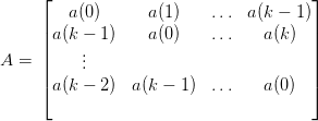
For example, a circulant matrix [HJ85] is useful for demonstrating a circular convolution using vectors:

(2.4)

and

(2.5)

where x and h are vectors of length k.

2.2.1 Baseband and Passband Signals

Signals on or around DC (direct current, or zero frequency) are called baseband signals while signals that are around a higher frequency carrier are passband signals. In general the baseband signal is complex, while the passband signal is real. It is common to shift a baseband signal, x_bb, to passband, x_pb, and vice versa. The relationships are defined as in [BLM04] and apply to both continuous and discrete-time (with some restrictions) signals:

(2.6)

where the common I (in-phase) and Q (quadrature) signals are just the real and imaginary parts:

(2.7)

and:

(2.8)

The factor is included so that the norms of the baseband and passband signals are the same.

As we will see in later sections, most physical layer processing is done on complex representations of baseband signals. Usually, this is the most convenient way to do things.

2.3 Linear Algebra and Matrix Techniques

Much of the machinery of any communication physical layer comes down to manipulation of finite length discrete time signals which are represented with complex vectors. Thus, it is incredibly useful to be comfortable with linear algebra and matrix techniques such as those described in [HJ85]. A few key points are provided here.

Special matrices are useful as operators when multiplied by vectors that represent signals. We start with the most common.

2.3.1 Matrix Definitions

2.3.1.1 Diagonal Matrix

The diagonal matrix,

(2.9)

is a square matrix that will scale each element of a vector. That is, for x = ^T ,

(2.10)

This most common diagonal matrix is the identity matrix, I, in which all diagonal elements are 1. Mulitplication by the identity matrix does not change the original matrix or vector:

(2.11)

and

(2.12)

2.3.2 Eigenvalues and Eigenvectors

2.3.3 Singular Value Decomposition

2.4 Finite Fields

I wrap up the this chapter with a quick summary of a set of concepts and techniques that are primary used in error correcting codes.

The most common field that we use every day is GF(2) (Galois Field of order 2) or binary logic. A field is closed under two operations. For binary logic, these are AND and XOR.

Chapter 3
Communication Theory Background

3.1 Mutual Information and Channel Capacity

The key problem in communication, in its most abstract form, is information from a transmitter, described by x, that is observed by a receiver as y. We assume x and y are random variables (or vectors of random variables) for which probability distributions are defined. From y, the receiver will attempt to do the best it can to determine x.

The mutual information between x and y is defined as:

(3.1)

where the base 2 is employed in the logarithm so that the units are bits.

Typically, the transmitter will employ a discrete alphabet for signaling, but the signal will be corrupted by noise in transmission. In many systems, the noise will be additive, white, and Gaussian. The resulting channel has the form:

(3.2)

where:

(3.3)

and N is zero mean with variance σ². X is a discrete random variable with uniform density:

(3.4)

and the density of Y given X is a Gaussian:

(3.5)

.

The capacity of the channel is defined as the maximum possible mutual information over all input densities:

(3.6)

The capacity is the highest rate at which error free transmission is possible over a channel. This is a topic that goes well beyond the scope of these notes. A good place to learn more is in [CT91]. Channel capacities are purely theoretical results, but, as we shall see later, they are immensely useful in understanding how well a practical system is operating.

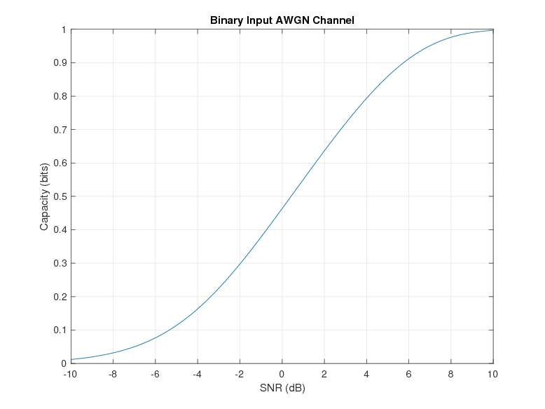
Let’s take a look at the capacity of a binary input AWGN channel. Binary phase shift keying (BPSK) with no intersymbol interference has this characteristic. We have two input symbols, −s and s. We first find

(3.7)

and so we can take the sum over the two values of X to determine the density of Y :

(3.8)

Then the capacity can be written as:

(3.9)

There is no closed form solution. However, the solution can be found by numerical integration. The signal to noise ratio in decibels will be:

(3.10)

and the capacity is shown in the figure below.

Figure 3.1

3.2 Detection Techniques

Mutual information and channel capacity set bounds on what is possible, but they don’t provide sufficient insight into how to reach that goal. Additional insight, as well as actual techniques, come from detection and estimation theory.

Given our received signal, y, we want to find an estimate of the transmitted message, x:

(3.11)

In fact, we want more than that. We want a good estimate, or, if possible an optimal estimate. But what is optimal?

The most basic and useful measure for optimality in communication is to minimize the number of errors we make. This isn’t as simple as it sounds because, as covered later, it might mean bit errors, symbol errors, frame errors, etc. For now, we can define:

(3.12)

and, correspondingly:

(3.13)

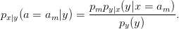
Minimizing the probabality of error is equivalent to finding the decision rule that maximizes the probability of correctly selecting the message that was transmitted given the received signal. The Maximum A posteriori Probability (MAP) decision rule is optimal [Lap09] [Gal08] in that it will minimize the probability of error. We can write the MAP rule as:

(3.14)

The rule is to look at the conditional probabilities for different transmitted signals x = a_m given the received probability density of the received signal y and select the one that is the largest.

In practice, it is often more common to employ a maximum likelihood (ML) detector. The ML decision metric is easier to compute. It can be derived from the MAP probability by:

(3.15)

The ML decision rule is then:

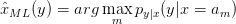(3.16)

3.3 Estimation Techniques

Communication problems are framed as estimating discrete random variables and sequences. However, that is only one problem that we need to solve in physical layer design. Real communication systems require estimation of non-random parameters, such as carrier frequency or the channel impulse response. There are many different techniques available, but most are based on least squares estimation or an approximation of least squares.[BF01][GL89]

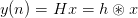
As an example, let’s examine channel impulse response estimation. A known baseband signal x is convolved with an unknown channel, h. The receiver observations are corrupted by noise:

(3.17)

The convolution can be expressed as a matrix-vector multiplication with X defined as:

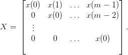(3.18)

The entire equation then takes the form:

(3.19)

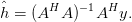
and the least squares estimate of h can be computed:

(3.20)

.

3.4 Channel Coding

Channel coding encompasses a set of techniques than can be used to maximize the error free transmission rate over a channel. This section provides a short background into the theory behind coding, while a later section decribes practical implementations that are used in real physical layers.

Classical coding include algebraic block codes and convolutional codes. These are traditional error correcting codes that have been in common use since the 1960s and are still used today. Modern coding refers to Turbo and Low Density Parity Check (LDPC) codes that can achieve higher performance.

In general, classical coding techniques are more amenable to analytical techniques than modern codes. This makes it easier to select a classical code and predict its performance. Also, classical encoding and decoding techniques are older, which means they are much less likely to be encumbered by intellectual property.

In contrast, it is almost always possible to design a better code with modern techniques and, for this reason, they are used in new high performance systems.

3.4.1 Classical Coding

3.4.1.1 Linear Block Coding

The mathematical theory behind linear block codes is vast and I only scratch the surface here. The standard definition for a linear block code ([LDJC04]) uses a (k,n) generator matrix, G. A length k message, u, is encoded into a length n codeword

(3.21)

where v is an n element row vector describing a codeword in a code C,

(3.22)

A (n − k,n) parity check matrix, H, is defined from the generator matrix via

(3.23)

and all codewords are part of the null space of H:

(3.24)

The elements of u, v, G, and H are from a finite field. Often it is GF(2) but other fields, such as GF(2^m) used in Reed-Solomon codes. In GF(2), multiplication is the common Boolean “AND” while addition is the Boolean “XOR”.

Since the code is linear, the all zeros vector is always a codeword. Furthermore, the sum of any two codewords is also a codeword.

The Hamming weight of a codeword, v is defined as the number of non-zero elements it contains, w(v). The distance between two codewords is defined as the number of elements in which they differ. This can be expressed as:

(3.25)

.

The most important property of a code C is the minimum distance between codewords. This determines how effective the code will be in detecting or correcting errors, d_min. The minimum distance is equal to the non-zero codeword with the smallest weight:

(3.26)

3.4.1.2 Convolutional Coding

3.4.2 Modern Coding

3.5 Sequences

Every physical layer design employs known sequences for estimating signal or channel parameters. This is commonly referred to as“receiver training”, i.e. the receiver employs the fact that it knows the sequence to determine a signal property, such as power level, frequency offset, or the channel the signal as passed through. Sequences are chosen for certain qualities that determine how well they perform for estimating parameters or how easy they are to use. Several common sequences are described in this section.

3.5.1 Barker Codes

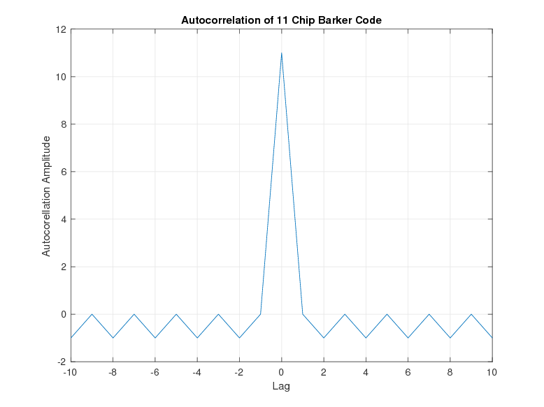
A Barker code is a sequence of binary symbols

(3.27)

with the property that the autocorellation at delay greater than zero is always less that 1. That is:

(3.28)

There are only 9 known Barker codes and the longest is of length 13. The length 11 Barker code is used as a spreading sequence in the original 1997 IEEE 802.11 standard:

(3.29)

Since the Barker sequence is binary, it is extremely simple to implement in both the transmitter as a modulator and in the receiver as matched filter. However, its use is limited because of the residual off zero autocorrelation terms. Figure 3.2

3.5.2 CAZAC Sequences

CAZAC (Constant Amplitude Zero Autocorrelation) sequences of arbitrary length with cyclic autocorrelation of zero for non-zero delay. This property makes them useful for synchronization and channel estimation. Implementation of these sequences is more complicated, however, because they are not drawn from a simple binary alphabet. The amplitude is always one, but the phase angle takes on values that are drawn from 2π, where N is the sequence length and m is an integer.

Even length CAZAC sequences can be generated with:

(3.30)

where N is the sequence length and M is an integer relatively prime to N. This type of sequence is often called a Zadoff-Chu sequence after [Chu72].

A PHY layer training field can be constructed for simplified channel estimation with a repeated CAZAC sequence. For example, the traing field:

(3.31)

passes through a linear channel h(k) and is corrupted by noise sequence n(k). Since the training sequence is repeated, the receiver observes a circular convolution of the CAZAC sequence and the channel as the second half of the training sequence is received:

(3.32)

(3.33)

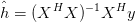
The matched filter for a(k), i.e. a^∗(k), applied to y(k), will yield a least squares estimator for h(k). This can be demonstrated by constructing the circulant matrix from a(k), i.e.

(3.34)

and noting that the least-square estimate of h(k) is as shown in 3.20:

(3.35)

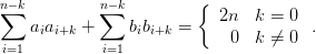
However, for any CAZAC sequence,

(3.36)

so

(3.37)

Thus, the estimator complexity is reduced from a matrix multiplication to a linear filter.

LTE systems employ CAZAC (Zadoff-Chu) sequences for primary synchronization of the user equipment (UE) from the basestation.[Ahm14]

3.5.3 Complementary Sequences

Complementary sequences provide many of the benefits of CAZAC sequences but employ binary alphabets like Barker Codes. To do this, the sequences must be used in pairs that provide good autocorrelation properties. The most common are those described by Golay [Gol61].

A pair of length n binary sequences, a and b, with a_i ∈{−1, 1} and b_i ∈{−1, 1}, are complementary if:

(3.38)

Golay sequences are employed in the phy preamble IEEE 802.11ad standard to facilitate low complexity synchronization and channel estimation at low signal-to-noise ratios.

Chapter 4
Channels and Impairments

(4.1)

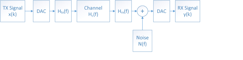
where y(t) is the received signal, x(t) is the transmitted signal, h(t) is the frequency selective channel, and n(t) is the Gaussian noise signal. Since the noise is typically introduced at the receiver front end, it does not experience the effects of the channel and can often be assumed to be white. White noise has the property of a flat spectrum, i.e. equal power per unit bandwidth. Perfectly white noise cannot exist, because it would have infinite power. However, it is a useful approximation to assume the noise is white over the band of interest. Typically, this would be over the Nyquist interval, (−,).

The simplest channel is one in which the frequency response is flat, i.e. h(t) = δ(t) and the noise is white. This is the AWGN channel mentioned in 3.1.

4.1 Frequency Selectivity

Frequency selectivity occurs naturally in channels and is designed into transmitters and receivers. Even if the channel itself is flat (i.e. a free space radio channel), the frequency response of components in the transmitter and receiver will create a frequency selective channel.

Figure 4.1

4.2 Time Varying Channels

4.3 Carrier Offset

4.4 Timing Offset

4.5 Phase Noise

4.6 Non-linearities

Chapter 5
Single Carrier Systems

5.1 Channel Estimation and Equalization

5.2 Decision Feedback Equalization

5.2.1 Fundamental Limits on use of the DFE

5.3 Fractionally Spaced Equalizers and Excess Bandwidth

5.4 Synchronization

5.5 Precoding

Chapter 6
Multi-carrier Systems

6.1 Multi-carrier Equalization

6.2 Multi-carrier Coding and OFDM

6.3 Synchronization

Chapter 7
Specialized Signal Processing Techniques

7.1 Signal Acquisition

7.2 I/Q Mismatch Compensation

7.3 Pre-distortion and Feed-forward Compensation

Chapter 8
MIMO Systems

8.1 Fundamental Techniques

8.2 Beamforming

8.3 Calibration

Chapter 9
Practical Channel Coding

9.1 Viterbi Decoders

9.2 Reed Solomon Decoders

9.3 LDPC Encoding and Decoding

9.4 Turbo Decoding

Chapter 10
Millimeter Wave Systems

Chapter 11
Example Physical Layers

11.1 802.11b

11.2 802.11ac

11.3 802.11ad

11.4 Bluetooth and Bluetooth LE

Chapter 12
Measures of Success

12.1 Complexity

12.2 Cost

12.3 Backward Compatibility

Bibliography